CJ Jiang posts photos

PCA for population genetics

10 December 2024

I’m interested in population genetics, the study of how populations evolve and how we can infer these evolutionary changes from looking at their genomes. Often, we wish to understand how individuals in a population genetically relate to each other, whether they’re split into two, clustered into groups, or something else.

One big problem, however, is dealing with the high dimensional nature of genomic data. A Single Nucleotide Polymorphism (SNP) is a site where individuals can differ. A population usually contains hundreds of sequenced individuals, each with tens, if not hundreds of thousands of SNPs. How would we even make sense of this data? Which SNPs should we use to compare individuals? If two individuals are similar at some SNPs but different at others, are they considered similar or different?

This is where dimensionality reduction techniques come in, the most popular of which for genomics is a Principle Component Analysis (PCA). Using PCA, we can infer simple relationships in high dimensional data by compressing it into two/three dimensions. By doing so, it is often (but not always) easier to see the relationships between observations. An example of the result of a PCA can be seen in Nelis et al. 2009 where a PCA was done for European human populations.

PCA example

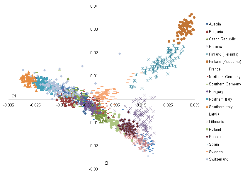
From this PCA, it seems that Finnish people are uniquely diverged from the rest of European populations.

Let’s say we monitor 5 SNPs across 3 individuals. For simplicity, let’s assume each SNP is biallelic (only having two possible states) and haploid (only having 1 copy).

Individual 1: 11111
Individual 2: 01001
Individual 3: 11011

We can encode these individuals as vectors in \(\mathbb{R}^5\).

\[x_1 = \begin{bmatrix} 1 \\ 1 \\ 1 \\ 1 \\ 1 \end{bmatrix}, \quad x_2 = \begin{bmatrix} 0 \\ 1 \\ 0 \\ 0 \\ 1 \end{bmatrix}, \quad x_3 = \begin{bmatrix} 1 \\ 1 \\ 0 \\ 1 \\ 1 \end{bmatrix}\]

Our dummy dataset only has 5 features, yet it is already impossible to visualize it in any meaningful way. The goal is to find a plane in \(\mathbb{R}^5\) to project our vectors onto. It is inevitable that projecting vectors from \(\mathbb{R}^5\) to \(\mathbb{R}^2\) will lose data, so we need to choose basis vectors that preserve the relationships between observations.

What does it mean to preserve relationships? Numerically, this means selecting the projection that preserves the most variance, retaining the spread and structure of the data.

First, we can combine our vectors into a \(3 \times 5\) matrix \(X\), where each row is an observation and each column is a SNP, or “feature”.

\[X = \begin{bmatrix} x_1^T \\ x_2^T \\ x_3^T \end{bmatrix} = \begin{bmatrix} 1 & 1 & 1 & 1 & 1 \\ 0 & 1 & 0 & 0 & 1 \\ 1 & 1 & 0 & 1 & 1 \end{bmatrix}\]

At this step, there are multiple ways to divide our data down into separate components, utilizing different decomposition techniques in linear algebra. We will do spectral decomposition/eigen decomposition, but know that other methods exist. We compute the covariance matrix \(\Sigma\), which simply describes how much each feature varies together with another feature. Intuitively, covariance is the same as correlation, but without being normalized into a unitless value.

First we center the data around 0 (\(X_c\)) by subtracting each observation by the mean across that feature.

\[X_c = \begin{bmatrix} 0 & 0 & 0 & 0 & 0 \\ -0.4 & 0.6 & -0.4 & -0.4 & 0.6 \\ 0.2 & 0.2 & -0.8 & 0.2 & 0.2 \end{bmatrix}\]

For a dataset with \(n\) features, the covariance matrix is an \(n \times n\) matrix, with each cell being the covariance of feature \(A\) with \(B\):

\[\text{Cov}(A,B) = \frac{1}{n-1} \sum_{i=1}^n (a_i - \mu_A)(b_i - \mu_B)\]

Finding the covariance matrix for our dummy dataset:

\[\Sigma = \begin{bmatrix} 0.0933 & -0.0733 & -0.04 & 0.0933 & -0.0733 \\ -0.0733 & 0.0933 & -0.04 & -0.0733 & 0.0933 \\ -0.04 & -0.04 & 0.16 & -0.04 & -0.04 \\ 0.0933 & -0.0733 & -0.04 & 0.0933 & -0.0733 \\ -0.0733 & 0.0933 & -0.04 & -0.0733 & 0.0933 \end{bmatrix}\]

Since the covariance matrix is a matrix of pairwise relationships, it is symmetric, meaning it is orthogonally diagonalizable and we can use spectral decomposition! By using spectral decomposition, we break down the covariances into 5 orthogonal eigenvector bases, (essentially, 5 directions the matrix acts in) with the eigenvalue being the scaling factor, i.e. how much variance in the direction of the eigenvector.

This gives us

\[\Sigma = \lambda_1 u_1 u_1^T + \lambda_2 u_2 u_2^T + \dots + \lambda_n u_n u_n^T\]

Since the eigenvalues describe how much variance is in the direction of each eigenvector, if we take the two eigenvectors with the largest eigenvalues (let’s suppose in our dummy case they are \(u_2\) and \(u_3\)), then, we have an orthogonal set of eigenvectors that point in the directions of greatest variance. These eigenvectors are called the principal components. We can then project our original data onto the space formed by these principal components.

\[y_i = \mathrm{proj}_{u_2} x_i + \mathrm{proj}_{u_3} x_i = (x_i \cdot u_2) u_2 + (x_i \cdot u_3) u_3\]

\(y_i\), though still an \(n\)-dimensional vector, now exists within the subspace of the principle components we have chosen.

To get the coordinates of the projected points in a 2D space, we get the scalar projections of the points with the principle components:

\[z_i = \begin{bmatrix} x_i \cdot u_2 \\ x_i \cdot u_3 \end{bmatrix}\]

Now each point \(z_i\) can be plot on a Cartesian plane, and we have completed a PCA!

Note: A PCA is not a magic wand that let’s us see into higher dimensions! It relies on the fact that a supposedly high dimensional data is not actually high dimensional, but really just 2 or 3 dimensional with some “noise” in other dimensions that we hope is not important.

We can evaluate the dimensionality of our data by looking at the eigenvalues, which each describes the variance explained by each basis vector. If they are uniform in value, then the data is spread across many dimensions and a PCA would be fairly useless. This would be the case if a population was panmictic (and in the case of bacteria, exchanges DNA frequently), for example. If 1 or 2 eigenvalues add up to more than 0.5, then a PCA may be a good choice.

Note 2: It is crucial that spectral decomposition gives us orthogonal vectors. Not only does this allow us to plot our new points in a Cartesian plane, but the highest variance principle components would be quite pointless if they were not orthogonal, since each axes would basically be the same.

References

Nelis, M., Esko, T., Mägi, R., Zimprich, F., Zimprich, A., Toncheva, D., Karachanak, S., Piskáčková, T., Balaščák, I., Peltonen, L., Jakkula, E., Rehnström, K., Lathrop, M., Heath, S., Galan, P., Schreiber, S., Meitinger, T., Pfeufer, A., Wichmann, H.-E., … Metspalu, A. (2009). Genetic structure of Europeans: A view from the north–east. PLoS ONE, 4(5). https://doi.org/10.1371/journal.pone.0005472
Jauregui, Jeff. 2012. “Principal component analysis with linear algebra”. Union College Website. https://www.math.union.edu/~jaureguj/PCA.pdf
Dubey, A. (2022, September 18). The mathematics behind Principal Component Analysis. Medium. https://towardsdatascience.com/the-mathematics-behind-principal-component-analysis-fff2d7f4b643